
Technology
A digital twin of the greenhouse: from a few plants in Omniverse to a whole greenhouse in Blender
Nov 20, 2026 · Vratislav Beneš
In Blender we built a photorealistic digital twin of a tomato and a pepper greenhouse, which we previously had in Omniverse. Neural networks trained only on its synthetic images recognise the concrete, the rails, the fruits and the plant stems in real photos from the robot. The twin can also simulate horticultural LED lighting. How did we do it, and why was it impossible three years ago? And where do real images still help?
Why a virtual greenhouse
Our Scout robot drives on the rails between the rows and its cameras capture the plants. But in a real greenhouse many things simply cannot be tried. A different type of rails or a different concrete on the main path? Those cannot even be changed. Different lighting, a young crop instead of a mature one? That takes time. Tomato brown rugose fruit virus (ToBRFV)? Nobody wants it in their greenhouse just to provide training data for AI. And many situations, such as a heavy infection or a diseased plant, cannot simply be waited for. Then there is the plain adaptation of the system to a new greenhouse or a new variety. And what if the customer has LEDs? There are more than enough problems with no training data.
So we wanted a digital space where we can test these variants easily. Where we set the time of day, the light (daylight and LED) or the plant height and immediately see what the robot's camera would see.
Speed is another big motivation. When the robot comes to a new greenhouse or a new variety, or meets a rare disease or pest, we do not have to spend months collecting and annotating images. We simply model the situation and prepare the system for it before it appears in the greenhouse at scale.
We made our first attempt three years ago in NVIDIA Omniverse. The virtual greenhouse worked, but on an RTX 4090 we could simulate only a few plants. A real row has hundreds of them. And a production greenhouse has 200 to 300 such rows.
Today things are different. Blender has MCP (Model Context Protocol), so a language model such as Claude, ChatGPT, Gemini or even a local model such as Gemma can model in it. Instead of clicking in the editor, you describe what you want, and the model writes and runs the code that builds the scene. The renders then run on a GPU server, not on a workstation.
Step 1: a single tomato plant
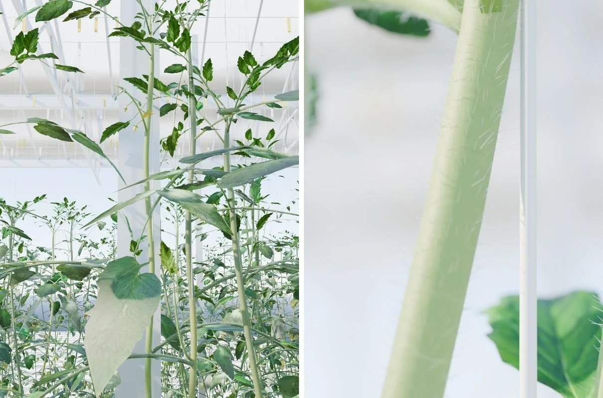
We started by importing into Blender a parametric tomato plant made by our colleague Adam. The very first result looked good.
Then we worked with the model on the look of the plant: the stem laid in the hooks and trained up a string, leaves made from photos of real leaflets, trusses from flowers to ripe fruits, hairs on the stem. We got to a point where we were not yet satisfied, but we were already extremely positively surprised how far one can get just by talking to the model.
Even a detail as fine as the hairs (trichomes) on the stem and leaf stalks can be modelled. For the robot this is not cosmetics: the hairs change how the stem reflects light and what its outline looks like in the camera image.
Step 2: a greenhouse modelled on reality
The next step was to put the plants into the environment where Scout actually drives. Following photos and videos from a real greenhouse, we built the scene: gutters with plants, rails between the rows, heating pipes, foil on the ground, the concrete main path, a Venlo roof, and the sun according to location and time. We also added the robot from its CAD model, people, lifts, trolleys and harvest crates.
The result again exceeded expectations. The twin has 26 + 26 rows, the scene builds in about 25 minutes and a Full HD frame renders in roughly 6 seconds. Compared to a few plants in Omniverse, that is a different world. For rendering and the subsequent training we now use a machine with NVIDIA RTX PRO 6000 Blackwell cards with 96 GB of VRAM, which handle even large scenes with thousands of plants.
To see how close we are to reality, we simulated two real videos from the robot: entering a row and driving along the main path. We measured the camera trajectory directly from the real video and replayed it in the twin.
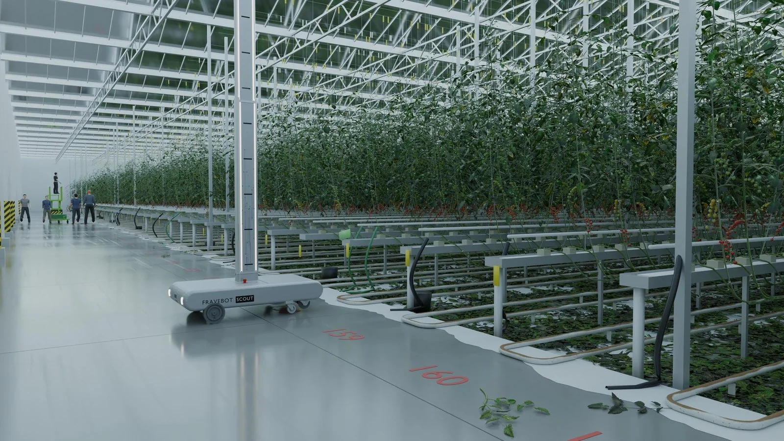
The twin also works as a simulator of artificial lighting. We place Philips luminaires with different spectrum recipes above the aisles, and the fruits and leaves change colour according to how they reflect that light. Horticultural LEDs are not just one colour: red, blue, white or far-red are mixed, and their ratio and output change during the day. From the same scene we get images for all these lights, so we can adapt the models to them before the robot ever arrives in such a greenhouse.
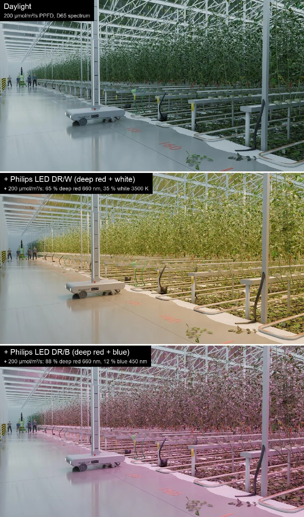
Scene parameters:
| daylight | + LED DR/W | + LED DR/B | |
|---|---|---|---|
| PPFD on the crop | 200 µmol/m²/s | 200 µmol/m²/s | 200 µmol/m²/s |
| spectrum (photon share) | D65 | 65% deep red 660 nm, 35% white 3500 K | 88% deep red 660 nm, 12% blue 450 nm |
| PAR radiation | 44 W/m² | 38 W/m² | 38 W/m² |
| energy per µmol of photons | 0.22 J | 0.19 J | 0.19 J |
| source | sun and sky | 528 modules 4.8 m above the floor | 528 modules 4.8 m above the floor |
The modules hang in a line above every aisle (1.6 m apart), one every 2.5 m. The coloured LED channels have a 20 nm FWHM. The colours are computed for the spectral sensitivity of the robot's IMX708 camera with its IR-cut filter at 655 nm. The Philips spectra are modelled from the manufacturer's descriptions for now; we will replace them with spectrometer measurements.
Step 3: synthetic data and the first models
A big advantage of a virtual greenhouse: with every image we get a precise mask of every object for free. Nobody has to trace the concrete, the rails or the fruits by hand. So we generated training data from the point of view of the robot's navigation camera, which sits about 20 cm above the concrete.
We trained the RF-DETR-seg segmentation network on them and ran inference on real images from the greenhouse. That truly took our breath away. A model that had never seen a real photo correctly found the concrete, the rails and the empty rows. Another model, also trained on synthetic data only, reliably recognises people, trolleys, lifts, crates and buckets in a real video.
When we added a smaller amount of annotated real images to the synthetic data, the results improved further. The test ran on real images from different days than the training data:
| what the model looks for | synthetic only (1,120 images) | synthetic + real images |
|---|---|---|
| concrete of the main path, IoU | 0.87 | 0.95 |
| rail in front of the robot, IoU | 0.80 | 0.90 |
| empty row, AP50 | 0.75 | 0.97 |
IoU tells how precisely the model's mask overlaps the manual annotation (1 = perfectly). AP50 is the object detection score (1 = all found with no false alarms).
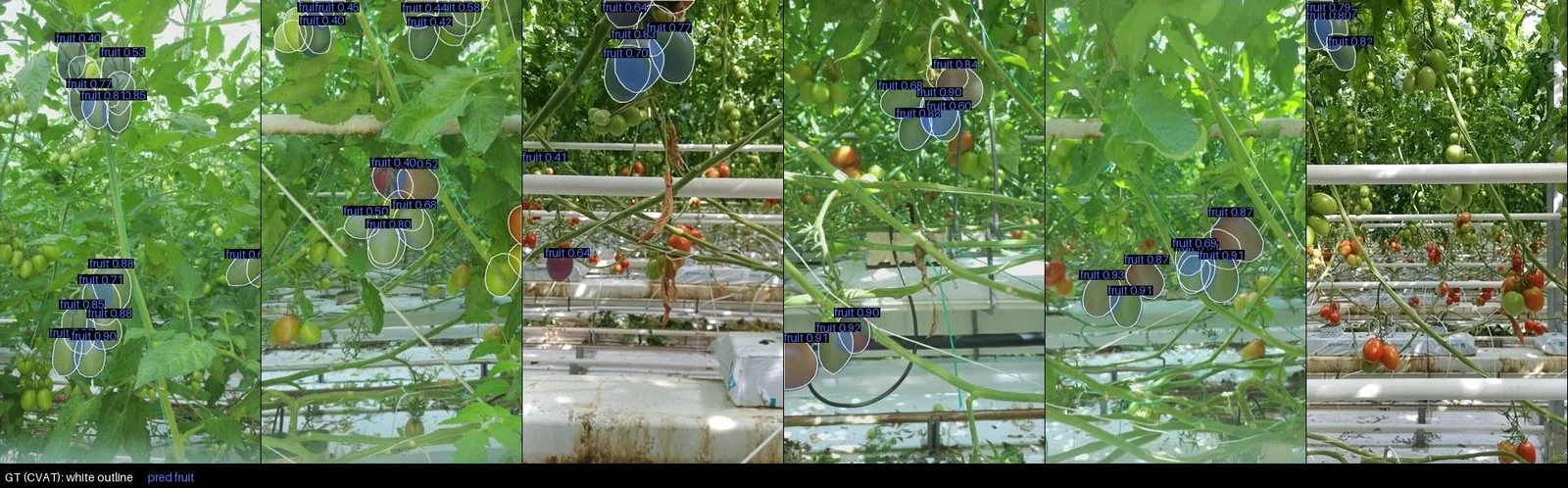
The same approach works for tomato fruits too. The synthetic fruit annotations match how people draw them in CVAT: only the fruits of the front plant next to the camera, and always the whole outline of the fruit, even where a leaf or a stem partly covers it. A model trained on just 1,944 synthetic images finds fruits in real photos with AP50 0.87, and with real images added 0.94:
| tomato fruits | synthetic only (1,944 images) | synthetic + real images |
|---|---|---|
| AP50 | 0.87 | 0.94 |
| IoU | 0.77 | 0.90 |
Step 4: textures from real annotations
In CVAT we have plenty of hand-annotated images from the greenhouse: outlined fruits, stems, leaves and flowers. We connected Blender to CVAT so that it cuts the textures out of these annotations by itself. The fruits in the twin thus have the colour and surface of real tomatoes at various stages of ripeness, the leaves the shape and veins of real leaflets.
Another source of textures is mobile phone photos sent to us by the growers themselves through our web app. A grower takes photos and describes a disease or pest, and our plant pathologist adds a detailed description of its behaviour: where on the plant it appears, what it looks like in each stage, how it spreads. The language model that builds the scene then has much better information to build it.
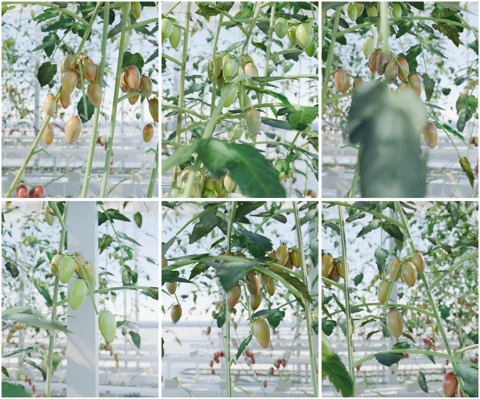
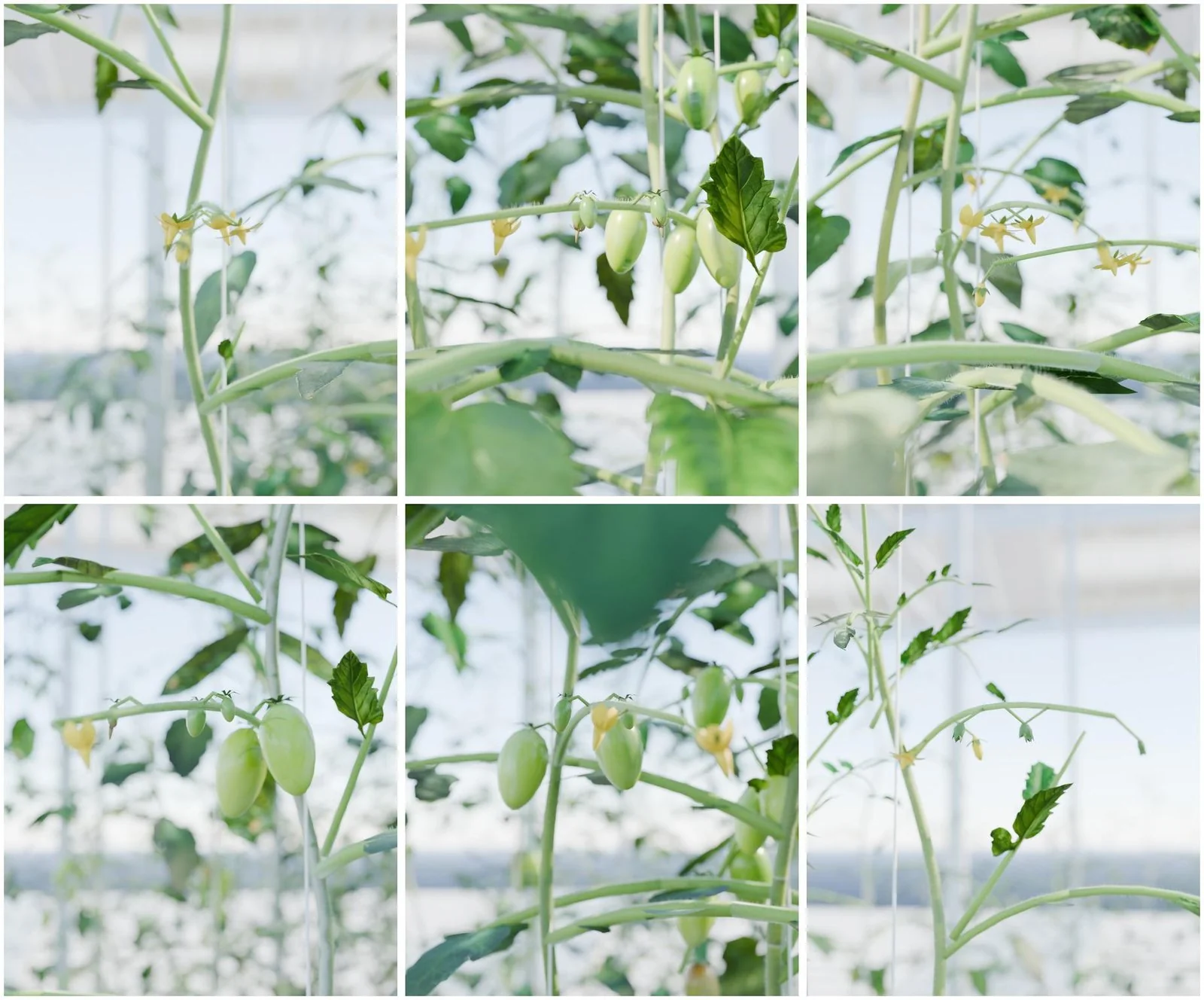
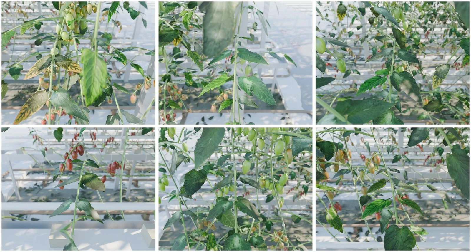
With the new textures we generated the data again, trained the models and compared them on real images from the greenhouse.
Stem bark cut out of the CVAT annotations helps mainly with old woody stems on the lower cameras.
Step 5: stems and the plant head
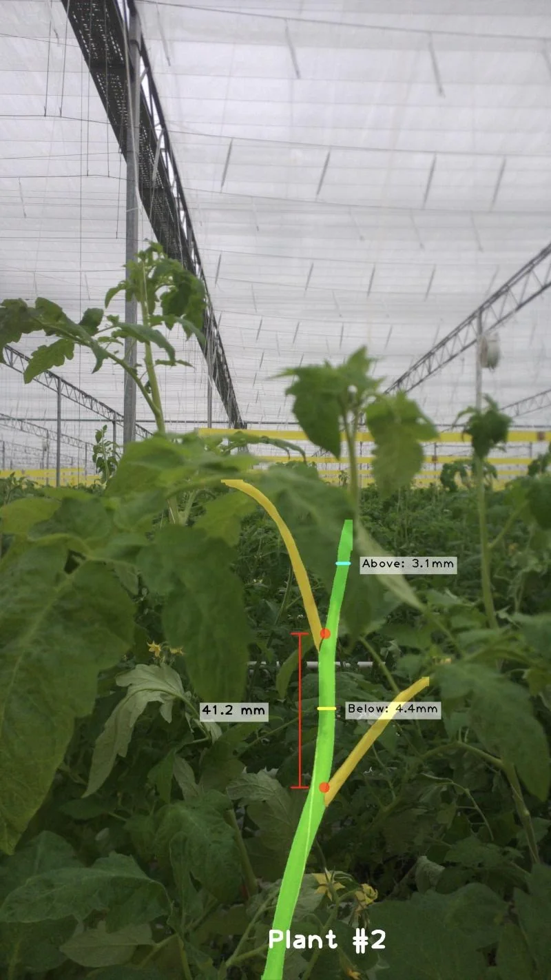
The hardest task is the stems, leaf stalks, strings and the plant head in images from the robot's upper cameras, from which crop growth is measured.
The synthetic scene for stems follows the geometry of row 280 in greenhouse 71, as measured by our colleagues who measure stems from the robot's cameras: the string is 0.47 m from the camera, the plants stand 31 cm apart and the stem is about 1 cm thick in its upper part. The whole row is lowered at once every two weeks, so the strings hang regularly and the plant head is sometimes in view of camera 07, sometimes 08. The annotations match how people draw them in CVAT: only the plants in the row next to the camera, a leaf stalk as the whole arc from the stem, and only the string the plant grows up.
The object counts per image are close between synthetic and real images; only leaf stalks are about twice as many in the synthetic ones:
| per image (cameras 07 and 08) | real images | synthetic images |
|---|---|---|
| stems | 1.1 | 1.3 |
| string pieces | 5.9–7.9 | 6.8 |
| leaf stalks | 3.3–4.6 | 7.3 |
| heads | 1.0 | 0.8 |
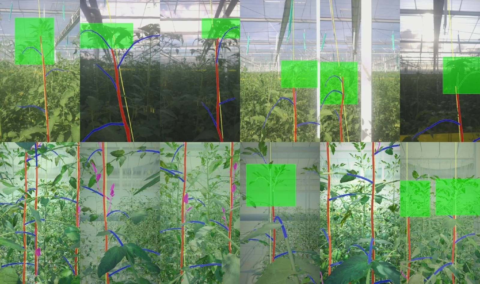
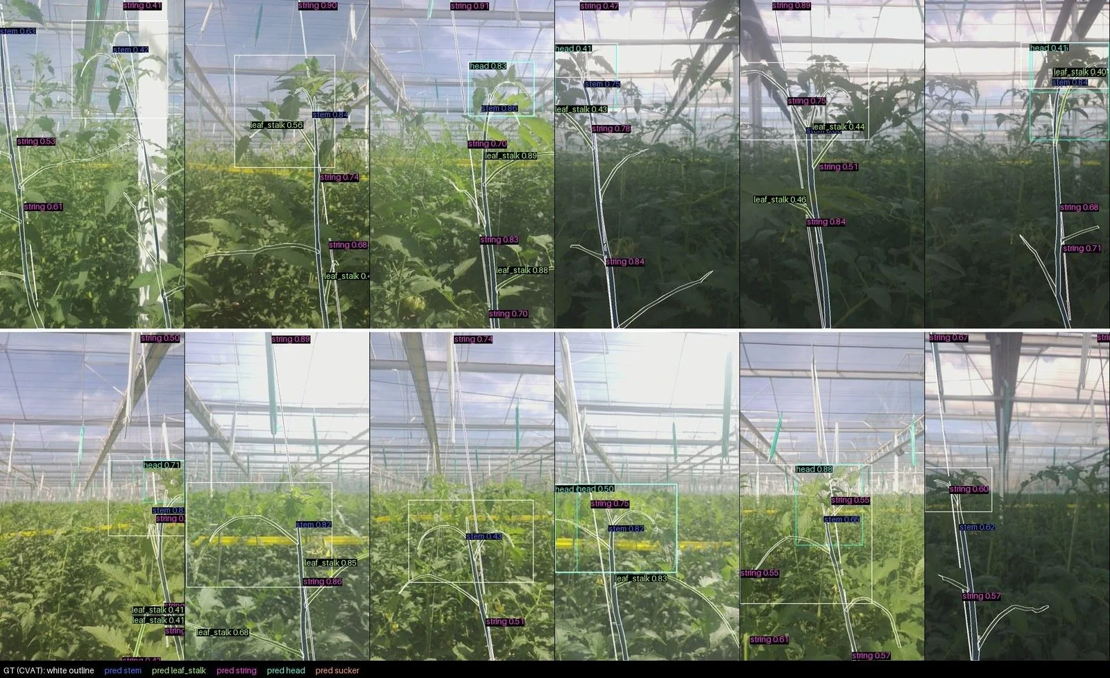
A model trained on this synthetic data alone, without a single real image, finds the stem in real images from cameras 07 and 08 with AP50 0.78 and 0.69. Leaf stalks and strings cannot yet be learned from synthetic data alone (AP50 below 0.1). One of the remaining differences is that the virtual plant has more leaves near the camera than the real one, and therefore more leaf stalks.
When we supplement 1,152 synthetic images with half of the hand-annotated real images and test on the other half, taken on different days, the model finds the stem near the head with AP50 above 0.9. Leaf stalks and strings are weaker so far:
| AP50 on real images | camera 07 | camera 08 |
|---|---|---|
| stem | 0.95 | 0.92 |
| leaf stalk | 0.17 | 0.23 |
| string | 0.22 | 0.22 |
For strings, the low AP50 is partly down to the metric. AP50 accepts a found object only if it overlaps the annotation by at least half, and it counts every annotated piece separately. In the annotation a string is split into 6–8 pieces depending on where leaves cover it, but the model draws it as one continuous strip. Pixel-wise overlap, which ignores the pieces, comes out at 0.35–0.44 for strings. For leaf stalks it is as low as AP50 (0.17–0.22); here the model still has real room for improvement.
Step 6: the pepper greenhouse
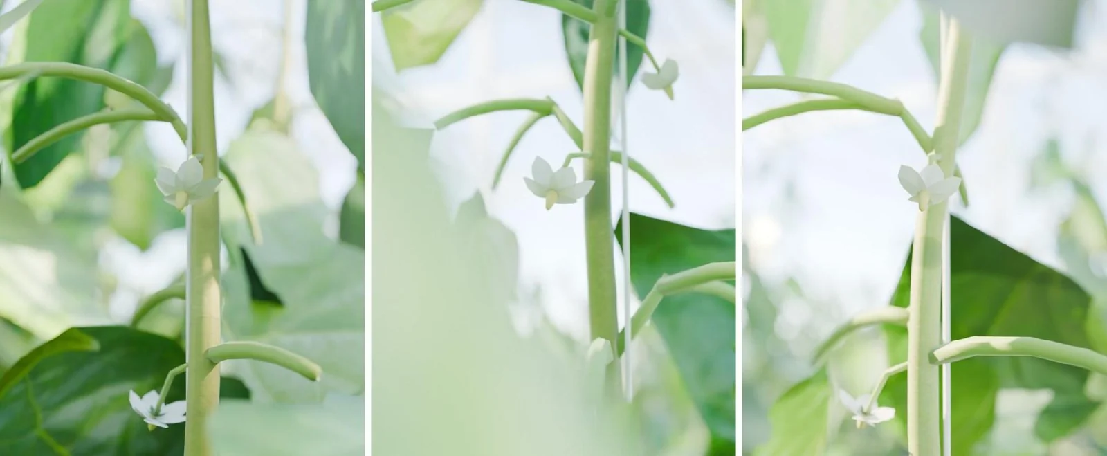
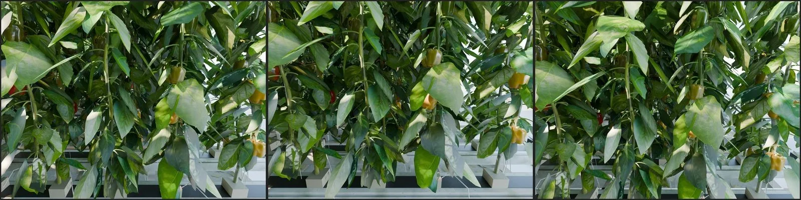
After the tomatoes we built a pepper greenhouse the same way. It is the same code with a crop switch, but almost everything is different. The bigger Scout 800 drives here on rails with an 80 cm gauge instead of 55 cm. Every row has two gutters side by side. The plants grow only upwards, each on two stems, up to about 3.5 m.
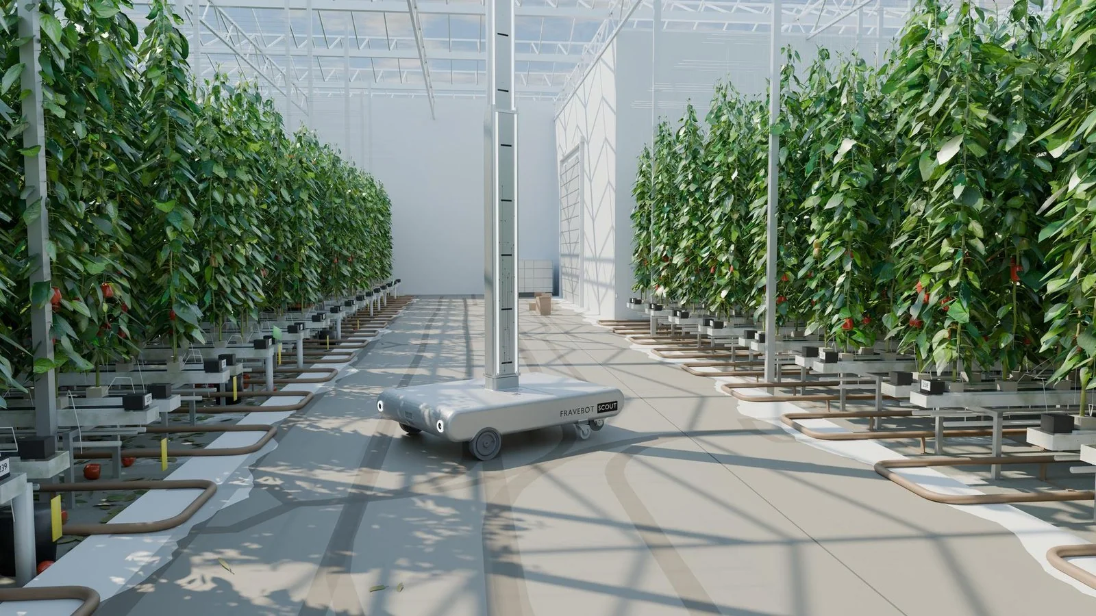
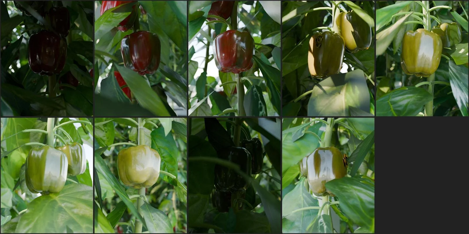
The pepper fruits come from a 3D scan of real peppers. The model can recolour them by ripeness from green to red or yellow and add disease spots from CVAT photos. We can also place the main pepper pest, a stink bug of the genus Nezara, into the scene in all its development stages.
Where we are heading
The goal is a greenhouse model on which we will train three things:
robot navigation: concrete, rails, row ends and above all foreign objects in the way, under different light and in different greenhouses,
plant measurement: stems, leaf stalks and heads in images from the upper cameras, from which crop growth is calculated,
disease and pest detection: cases that are rare in real data and therefore hard to collect and annotate by hand.
For navigation the twin matters most. In a real greenhouse the robot meets boxes left on the concrete, buckets, trolleys or a worker kneeling at a row. Such situations are rare in real recordings and cannot safely be staged on purpose. In the twin we prepare them as scenarios in any number and variant.
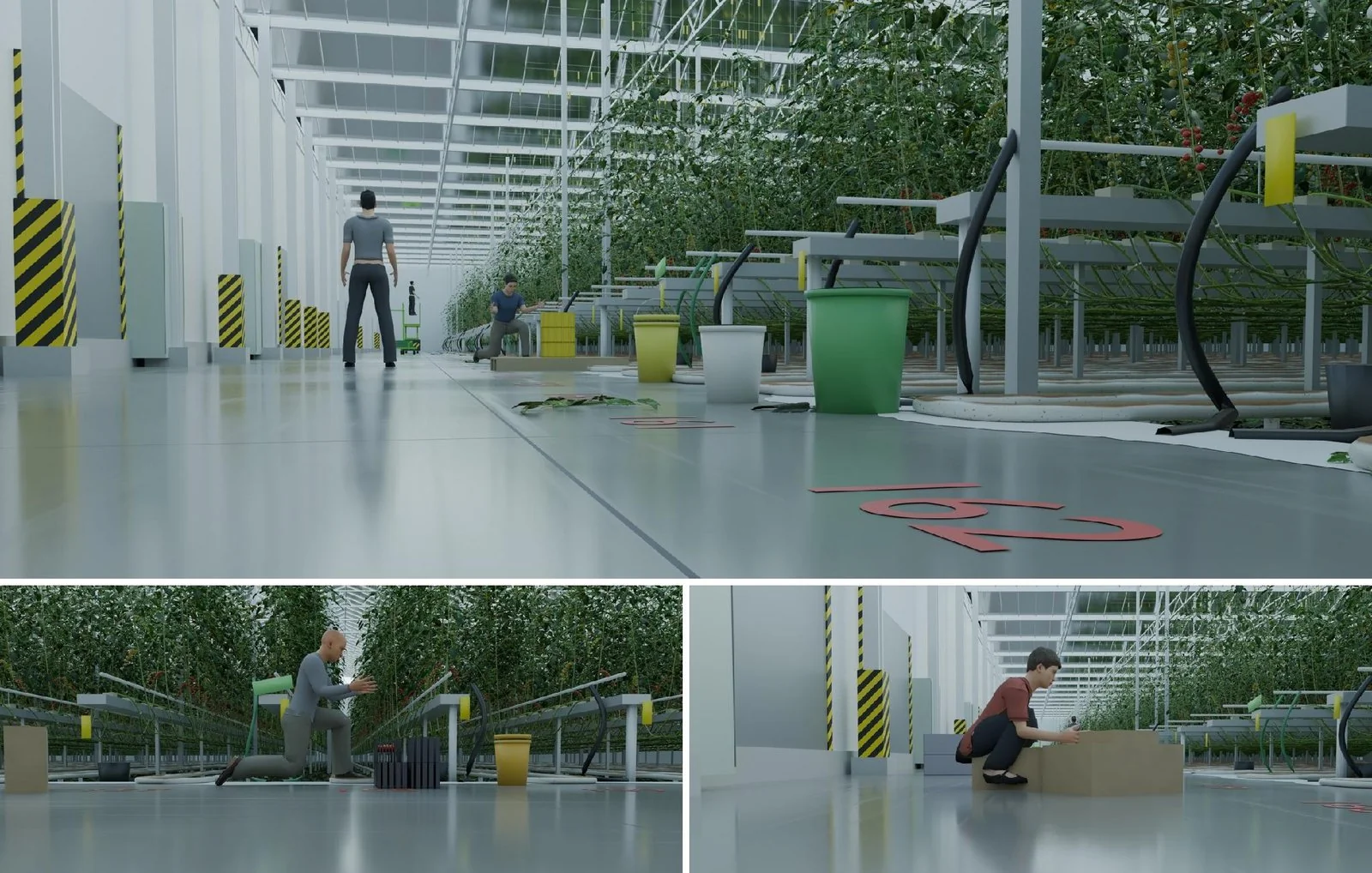
What this looks like in reality is shown by a video from the robot in the Čerstvě utrženo greenhouse:
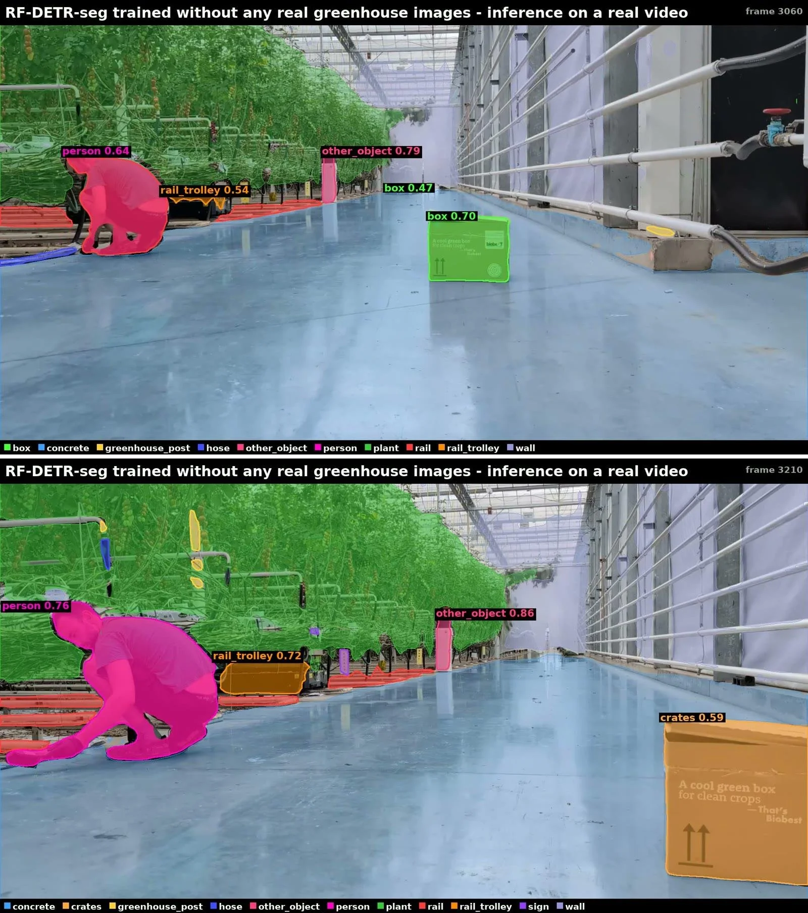
From these scenarios we will generate data and train two models to control the robot: RF-DETR-seg recognises from the image what is in front of it, and a language model with a LoRA adapter decides whether to drive around the object, wait, or stop and report it.
The robot also has physics in the twin, simulated in MuJoCo. So we can test its control in the virtual greenhouse before the robot drives into a real one.
Next step: the twin will regularly compare images from the robot's passes with its own renders and tune itself based on the differences, so that it matches the current state of the crop.
Three years ago we hit a limit of a few plants. Today we have entire greenhouses, and most of the work of building them was done by a language model in Blender.